Archive for the ‘Packet Analysis’ Category
Wireshark tid-bit: Looking for the smoking gun
It’s not always the network which is at fault but it is usually the network that is the assumed culprit. Wireshark can be a vital tool when troubleshooting difficult scenarios or prove that the network is not root cause. The purpose of this post is to ask questions and promote out of the box thinking when troubleshooting with Wireshark. Some common problems:
- The network is slow / This file transfer is slow
- My application responds after X seconds
- This application or agent is not working
These are very broad problem statements and depending on how familiar you are with the configurations and infrastructure, these can sound like daunting tasks to troubleshoot. At least until we start asking more questions and begin gathering the information we need to start troubleshooting. On occasion it is easier to capture packets on the source and destination endpoints then see what the packets tell us, will the packet capture align with the problem or will the packets point us in another direction?
When using Wireshark to troubleshoot such a board and undefined problem, where do you start? Wireshark is great at collecting details, Wireshark also presents all this information to us in an organized and digestable fashion. It’s up to us as network professionals to solve the mystery. Next up we’ll discuss some key items that will help expedite the troubleshooting process and make you more comfortable performing and reading packet captures. We will also ask some thought provoking questions to involve not just network-related technologies and issues.
Capture points and filtering options
The capture point is the foundation of your upcoming analysis. If you are not capturing at the correct spot (or spots) any future protocol analysis will either make the troubleshooting process more difficult and time consuming or you may find yourself going down the wrong path. It is always a good idea to review and understand the traffic flow which you are troubleshooting. Then ask yourself, will traffic be passing through my capture point? Could this traffic flow take another network path? Could another technology such as Virtual Port-Channel (vPC), Virtual-Chassis, load-balancers, load-sharing, ACLs (it can become quite a large list) be causing traffic to flow in another direction or drop the traffic flow all together? Depending on the size of the infrastructure is it possible to walk the path of the packet, following MAC, ARP, and routing tables?
Capturing at the right point is half of the battle, the next big question is what kind of capture filter do you need? Should you just capture everything passing through the interface in question? Some items to consider:
- If you perform an unfiltered capture and capture all the details:
- Will you create a performance bottleneck? Packet capturing can be resource intensive impeding network performance for production traffic flows.
- Will the packet capture be usable? The larger the packet capture the more time it takes to filter and analyze. You need to start filtering the conversation at some point either pre- or post- capture. Having all the data is great but will it be helpful?
- If you do decide to filter your capture what is your criteria?
- Source and Destination are always valuable but will that show you the entire picture? Will you see DNS resolution? Do you need to be aware of any HTTP redirects?
Timestamps
Being mindful of the timestamps logged in a packet capture, this information can help identify a wide array of different issues. Wireshark captures multiple timestamps, like almost every other field in the packet you can turn that field into a column this allows you to quickly identify gaps in time. You can take this a step further by marking a ‘reference’ packet allowing you to see the time delta from the reference packet. This can be useful when determining how long a requests takes or how long it takes a TCP handshake to complete.
e.g.: Why did the application server take 32 seconds to start transferring data? What was occurring during that 32 second gap? Perhaps there was a delay in receiving traffic from a backend database? Did you capture the backend flow too? Typically when a database is waiting on a transaction to complete you may see ‘keep-alive’ packets allowing the TCP connection to remain open/active while backend tasks are being performed. If you are troubleshooting a performance issue and see ‘keep-alive’ packets your next step may be to understand why the request is taking so long. Continuing with the database example, does a query need to be updated? Is the database fragmented? Does the server need additional resources (CPU/Memory/Disk/etc)?
Source and destination details
Don’t discount the source and destination details of the conversations. These details allow you to confirm the traffic is flowing the way you expect it to be going.
- MAC address – Does the source and destination MAC addresses line up with the expected network interfaces? Could the traffic be going a different path? Is there a misconfiguration causing traffic to flow over a different interface?
- I have seen colorful packet captures when LAG is enabled on the server-side but not on the network side. (This was not 802.3ad LACP)
- Dot1Q and IP details – Are you seeing the expected VLAN tags? Are any device dual-homed on multiple networks and could traffic be routed over an unexpected or different interface?
A packet capture can clearly show you what is happening, once you see what is happening you can then ask the question: Why is this happening? e.g.: A device receiving a packet on one VLAN but the response is received on a different VLAN, why is the response appearing on different network than which is was received?
Firewalls for instance allow you see packets getting ‘dropped’ or hitting the ‘bit bucket’, if you capture on both the rx and tx you expect to the see the same Dot1Q information, however if you find packets in the drop log with a different Dot1Q header than expected you can assume asymmetric routing and that may lead you to your root cause.
IP and TCP Options:
IP and TCP options provide an abundance of information about both the endpoints and the conversation:
- IP Length – The size of the packet can help identify packet loss involving MTU and fragmentation related issue.
- Fragmentation – What is the status of the DF-bit? Are overlays in play? How about Jumbo frames? Do you see certain packet size being transmitted from the source but not arriving at the destination? Do you need to move you capture point to identify the source of packet loss?
- Window Size and MSS – Much less a problem these days but does the TCP session have the appropriate TCP MSS and Window size are these setting being manipulated by a load balancer?
- IP Identifier – The IP ID field can be invaluable in the right scenario, especially when troubleshooting switching loops, routing loops, or even software bugs. I’ve done a previous write-up of the IP ID field and therefore won’t be going over the details again but I recommend giving it a quick read before finishing up here.
TCP Flags:
How is TCP behaving? Are you seeing the entire 3-way handshake? Besides capturing at the proper locations you also want to make sure your timing is correct, starting your capture before handshake occurs is vital to understanding the whole picture. The TCP handshake will include items discussed in the previous section such as the Windows Size and MSS, following the window size of a conversation may provide insight into packet loss or buffer issues on one of the endpoints. How about RST packets? It’s important to understand the application, some applications may not be coded properly and rely on RST packets to end connections as opposed to graceful closures with a FIN / FIN+ACK handshake. The last thing you want to do is go down the wrong path and assume something is wrong when it is indeed working as intended. (it may not be optimal but it may be as intended)
Protocol Dependancies
I briefly touched on this earlier in the post, it is good to see the full picture and follow the application / process in its entirety for example:
- When troubleshooting a connection issue are you are capturing the DNS resolution too?
- If you troubleshooting IP Storage or IP File access are you seeing any Kerberos or ticket authentication?
- Are you seeing a successful TLS handshake if you are working with a secure connection?
- In a security-conscience world do you see the RADIUS communication when troubleshooting device onboarding issues?
This post asked a lot of questions, as mentioned at the start this was aimed to provoke that out-of-the-box thinking: Am I troubleshooting this properly? Am I looking at the right pieces? Is there more to this issue than what I am considering? Hopefully some of these questions and examples did just that. I have other Wireshark posts on this blog, many of which are still valid after all these years, some stand-out ones to assist with troubleshooting:
As always, happy hunti…I mean troubleshooting!
As you can tell by my typos, grammar, sprinkled in references, and humor this post was written without the help of Artificial Intelligence (AI). These are my loosely organized ramblings.
Wireshark tid-bit: Quickly gathering the contents of a PCAP.
I don’t know about you but when I find myself performing packet captures and analyzing PCAPs I usually only know the symptoms of the issue I am attempting to troubleshoot. IE: Connection timeouts, slow response, long transfer times, etc. I usually don’t know much more than that, only in rare occasions do I get a heads up and insight into the behaviors of the application I am trying to troubleshoot. For all the other situations I need to rely on the PCAPs and interpret what and how the applications are communicating. Whether or not the application is behaving properly and performance is as it should be or if there is indeed something amiss somewhere.
Now for me the easiest way to do this is by using the reviewing the ‘Summary’ page under the ‘Statistics’ menu. A sample summary page is below:
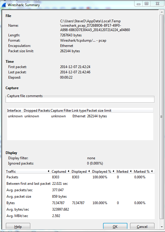
A few great call-outs from this screen:
- Packet Size Limit -Knowing whether or not the packets within the capture were sliced after the first so many bytes is important to know, as sometimes you might not see the entire TCP header or wireshark will start classifying the packets as malformed. Although you will also see a ‘Truncated’ message within the packet indicating the packet was sliced.
- First Packet, Last Packet, & Elapsed time -Matching up the time of a packet capture with when the particular issue occurred is crucial, after all you don’t want to find yourself analyzing the wrong capture. The Elapsed time is important to make note of as this give you the ability to establish a baseline, knowing how long a process takes can you help you identify an issue or identify expected behavior in the future.
- Avg. Packet Size – Depending on what you are trying to troubleshoot the average packet size can be a quick indicator in regards to whether or not your fully using the MTU an your network. If you are troubleshooting data transfers normally you would expect the Avg. Packet to be quite large. If you see exceptionally small packet sizes data transfers may take a lengthy amount of time due to the increase TCP overload and normal L3 forwarding. Same goes for the Avg Mbit/sec, if you have large packets flowing you can expect to see a higher throughput rate, and the opposite for lower packet size rate.
The next spot that is worth checking out is the ‘Conversations’ which is also found under ‘Statistics’ this quaint little window gives you a brief overview of any Source/Destination devices identified within the capture. From an L2 Ethernet perspective up to a L4 TCP/UDP Perspective allowing you see what end points are really involved with this communication along with how much data was sent, the length of time the connection, etc. It’s not completely unheard of for applications to communicate with other devices (Web Servers, DB Servers, File Servers, Other App Servers) to perform whatever tasks it is trying to perform and it could be very possible this third server may or may not be slowing down the process.

So by using these two windows in Wireshark you’ve identified the following:
- The length of time the process take. – Found in the elapsed time of the capture, as long as the entire process was captured that is.
- The endpoints involved with this communication. – Remember it is important to cut down as much background noise as possible.
- How much data is transferred and at what size & rate. – This can very helpful when working data transfers.
Wireshark Tid-bit: What does the IP Identification field tell us?
There are many different fields in the various headers we get to examine during packet analysis, one of the most overlooked field is the IP Identification field. This simple 16-bit field is displayed in Hex and has a few different uses, most importantly:
- Identifies fragmented packets.
- Identifies the individual packets that the sender transmits.
How does this help us?
- Well, by reviewing the IP Identification numbers you can easily identify which packet was dropped in the conversation, by comparing the packet captures from two different capture points.
- This field can also give us a glimpse at how busy the end-devices are. The IP Identification field will increase by ‘1’ for every packet from the sender. Remember the IP ID Value is specific to each individual and not to a specific conversation. If you are following a specific conversation we may see consecutive IP ID #’s or we could see large jumps in the IP ID # intervals. Depending on the numbers this could tell us if the end-devices could be overloaded, or under-utilized and depending on the situation that could point us to a smoking gun.
- If the packets get fragmented they will have the same IP ID number, the Fragment Offset field will also be set as well. This is helpful in following a conversation over particular link changes.
- Seeing the same IP ID #’s in the same packet capture could also identify switching or routing loops within our network. The IP ID #’s will always increase, seeing the duplicate numbers means were are seeing the same packet more than once. The first thing you want to do is verify your capture point is functioning properly and make sure your capture point is in the right spot. Once you verified that it’s time to go hunting for the loop.
Quick Example:
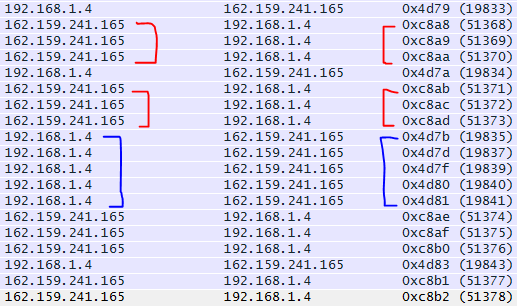
By reviewing the IP ID numbers of the packets what can we tell about this conversation with Wireshark.org?
- All the IP ID #’s are unique, no routing/switching loops
- The IP ID #’s are pretty consecutive on both sides of the conversation. Showing both endpoints are not being highly utilized at this point in time. In fact there are one or two gaps on the 192.168.1.4 side of the conversation showing that endpoint is a little busier than 162.159.241.165
Wireshark tid-bit: Packets larger than the MTU size.. why, how?
Ever so often when I was doing some packet analysis I would come across systems that were sending packets larger the Ethernet MTU of the segment. Or so I thought those packets were getting transmitted, eventually I finally figured out why I was seeing packets with an increased packet size.
The answer was large segment/send offload (LSO) – When this feature is enabled it is the responsibility of NIC Hardware to chop up the data ensuring why it conforms to the MTU of media/network segment.

Now that we know why we are seeing these large packets, the next part of the question is how are we seeing these large packets in Wireshark. Well, Wireshark relies on WinPCAP or LibPCAP depending on your platform, these two tools capture the packets just before the packets hit the NIC Card and get transferred to the actual network.

The above image is from Winpcap.org, showing the kernel level NPF just above NIC Drive, thus explaining how Wireshark is able to see the larger traffic. Before it hits the NIC Driver and gets segmented due to its LSO capabilities.
Winpcap.org – Winpcap Internals
Use your router to perform packet captures.
For quite some time now Cisco routers have had a feature known as EPC embedded packet capture, this feature allows you to perform packet captures directly on the interfaces making this one of the most useful features Cisco could implement (in my own opinion of course), a few things you can do with this feature:
- Listen to VoIP calls to verify quality
- Verify packet markings
- Troubleshooting connectivity issues
- and so on.
The best part of this, is the fact the configuration is fairly simple and you can begin capturing packets with just a few simple commands.
Here is a quick outline of the process:
- Create a buffer point
- Create a capture point
- Tie the buffer point & the capture together
- Start the capture
- Stop the capture
Now to dive a little deeper!
The buffer point is memory used to hold the packets captured and as we all know Cisco devices have a finite amount of memory on them and we would not want a packet capture to completely utilize all the space and cause other issues. So this where we limit what gets put in the buffer. On top of that we can also set filters based off an access-list in order to limit the packets we will capture, since in many cases we would not want to capture all the data traversing the router.
![]()

Buffer Point Options
Next we need to specify the capture point, this is where we specify the interface we want to capture on and in which direction we want to capture in. One thing you will need to specify is if you want to capture CEF or process switched traffic, this option in itself I think I just awesome (Of course most of the time you will capture CEF switched packets) but it’s nice to have the option. One thing I want to throw out there is yes you can capture on sub-interfaces.


You have the option to capture both IPv4 & IPv6 traffic
Now that we have created the capture point and the buffer point, we need to tie them together, this done with the following command:
![]()
All we need to do now is start then stop the capture, with the following command:

You can either manually stop the capture, or use one of the various options in the buffer point to trigger the capture to automatically stop.
Once the capture is complete you will most likely want to export the capture off the router and to your own workstation for deeper analysis in Wireshark or Omnipeek. You can export the capture off box by using protocols like TFTP or FTP, or even export the file directly to flash and come back to it later.
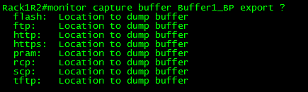
Buffer export options
Just think about the doors this opens for troubleshooting those odd random issues where you only wish you could capture the traffic for further analysis now you can!
Also think about the other cool things you can do with EPC:
- Utilize EPC on multiple interfaces at the same time, with multiple capture & buffer points. (Check out this page from Cisco)
- Use EPC in conjunction with kron jobs or EEM applets to perform on-demand packet captures.
- Much more
Let’s check out an IPv6 header.
I touched on the IPv6 addressing scheme a few weeks ago before and I wanted to continue the trend into a few more IPv6 related posts but that last IPS post spiked my interest, so I had to publish that one. Now we know the addressing scheme is different in IPv6 but what about the packet format? Obviously the packet headers will be larger because the source and destination addresses within that header are now 128 bits but let’s see what else we have in the IPv6 header:

Now that doesn’t look too intimidating right? I think that looks a little simpler compared to the IPv4 packet header. Now let’s see what we got going on here:
- Version: This field is in an IPv4 packet and simply tells us what version of IP we are running. Since this is an IPv6 packet it’s going to have a value of 6
- Traffic Class: This is the equivalent of the DiffServ/DSCP portion of the IPv4 packet which carries the QoS markings of the packet. Just like in IPv4 the first 6 bits are designated for the DSCP value, and the next 2 bits are for ECN (Explicit Congestion Notifications) capable devices.
- Flow Label: This field is 20 bits long and is defined in RFC 6437, I’ll admit finding information about the flow label is tough, but the RFC state this field could be used as a ‘hash’ for the routing devices look at and make forwarding decisions based on the field’s value. Its intention is for stateless ECMP (Equal Cost Multi-Path) or LAG mechanisms, but we will have to see how different vendors implement this feature. I’d take guess that IPv6 CEF will use the flow label, but I’ll have to wait and see.
- Payload Length: Specifies the size of the data payload following the IPv6 header.
- Next Header: This field is 8-bits and specifies the layer 4 transport protocol which follows the IP header. These values are hex format as well, you’ll notice ICMPv6 has a value of 0x3a, IPv6 protocol numbers use the same numbers that were used in IPv4. IANA’s list of protocol numbers can be found here.
- Hop Limit: This is also an 8-bit field and replaces the TTL field that was in the IPv4 header. Each hop decrements the hop limit value by 1 and when the hop limit reaches Zero the packet is discarded.
- Source/Destination: This should go without saying but it tells you the source IPv6 address of the packet and the destination IPv6 address this packet is destined to. As you would expect both of these field are 128-bits each.
So there is a snappy run down of the IPv6 IP Packet header, I think it is actually simpler than the IPv4 IP packet headers but don’t tell that to a Cisco router. Remember these packet headers are considerably larger than their IPv4 counterparts so it takes more processor power to process IPv6 packets which is not a problem for the ISR G2’s we have todays but it is something you might want to keep in mind when run IPv6 on older hardware.
Now back to CCIE: R/S Labbing I go!

